Previous posts in this series:
Silent Duels and an Old Paper of Restrepo Silent Duels—Parsing the Construction Silent Duels—Constructing the Solution part 1
Since it’s been three years since the last post in this series, and the reason for the delay is that I got totally stuck on the implementation. I’m publishing this draft article as partial progress until I can find time to work on it again.
If you haven’t read the last post, please do. Code repo. Paper I’m working through. In this post I make progress on implementing a general construction of the optimal strategies from the paper, but at the end the first serious test case fails. At the end I’m stuck, and I’m not sure what to do next to fix it.
Refactoring
Let’s start by refactoring the mess of code from last post. Now is a good time for that, because our tinkering in the last post instilled certainty we understand the basic mechanics. The central functions for the generic solution construction is in this file, as of this commit.
We’re using Sympy to represent functions and evaluate integrals, and it helps to name types appropriately. Note, I’ll using python type annotations in the code, but the types don’t validate because of missing stubs in sympy. Call it room for improvement.
from sympy import Lambda
SuccessFn = NewType('SuccessFn', Lambda)
@dataclass
class SilentDuelInput:
    '''Class containing the static input data to the silent duel problem.'''
    player_1_action_count: int
    player_2_action_count: int
    player_1_action_success: SuccessFn
    player_2_action_success: SuccessFn
Now we turn to the output. Recall, a strategy is a partition of $[0,1]$ into $n$ intervals—where $n$ is the number of actions specified in the input—with a probability distribution for each piece of the partition. This suggests a natural breakdown
@dataclass
class Strategy:
    '''
    A strategy is a list of action distribution functions, each of which
    describes the probability of taking an action on the interval of its
    support.
    '''
    action_distributions: List[ActionDistribution]
And ActionDistribution is defined as:
@dataclass
class ActionDistribution:
    '''The interval on which this distribution occurs.'''
    support_start: float
    support_end: float
    '''
    The cumulative density function for the distribution.
    May be improper if point_mass > 0.
    '''
    cumulative_density_function: Lambda
    '''
    If nonzero, corresponds to an extra point mass at the support_end.
    Only used in the last action in the optimal strategy.
    '''
    point_mass: float = 0
    t = Symbol('t', nonnegative=True)
    def draw(self, uniform_random_01=DEFAULT_RNG):
        '''Return a random draw from this distribution.
        Args:
         - uniform_random_01: a callable that accepts zero arguments
           and returns a uniform random float between 0 and 1. Defaults
           to using python's standard random.random
        '''
        if self.support_start >= self.support_end:  # treat as a point mass
            return self.support_start
        uniform_random_number = uniform_random_01()
        if uniform_random_number > 1 - self.point_mass - EPSILON:
            return self.support_end
        return solve_unique_real(
            self.cumulative_density_function(self.t) - uniform_random_number,
            self.t,
            solution_min=self.support_start,
            solution_max=self.support_end,
        )
We represent the probability distribution as a cumulative density function $F(t)$, which for a given input $a$ outputs the total probability weight of values in the distribution that are less than $a$. One reason density functions are convenient is that it makes it easy to sample: pick a uniform random $a \in [0,1]$, and then solve $F(t) = a$. The resulting $t$ is the sampled value.
Cumulative density functions are related to their more often-used (in mathematics) counterpart, the probability density function $f(t)$, which measures the “instantaneous” probability. I.e., the probability of a range of values $(a,b)$ is given by $\int_a^b f(t) dt$. The probability density and cumulative density are related via $F(a) = \int_{-\infty}^a f(t) dt$. In our case, the lower bound of integration is finite since we’re working on a fixed subinterval of $[0,1]$.
The helper function solve_unique_real abstracts the work of using sympy to solve an equation that the caller guarantees has a unique real solution in a given range. It’s source can be found here. This is guaranteed for cumulative distribution functions, because they’re strictly increasing functions of the input.
Finally, the output is a strategy for each player.
@dataclass
class SilentDuelOutput:
    p1_strategy: Strategy
    p2_strategy: Strategy
I also chose to make a little data structure to help maintain the joint progress of building up the partition and normalizing constants for each player.
@dataclass
class IntermediateState:
    '''
    A list of the transition times computed so far. This field
    maintains the invariant of being sorted. Thus, the first element
    in the list is a_{i + 1}, the most recently computed value of
    player 1's transition times, and the last element is a_{n + 1} = 1.
    This value is set on initialization with `new`.
    '''
    player_1_transition_times: Deque[Expr]
    '''
    Same as player_1_transition_times, but for player 2 with b_j and b_m.
    '''
    player_2_transition_times: Deque[Expr]
    '''
    The values of h_i so far, the normalizing constants for the action
    probability distributions for player 1. Has the same sorting
    invariant as the transition time lists.
    '''
    player_1_normalizing_constants: Deque[Expr]
    '''
    Same as player_1_normalizing_constants, but for player 2,
    i.e., the k_j normalizing constants.
    '''
    player_2_normalizing_constants: Deque[Expr]
    @staticmethod
    def new():
        '''Create a new state object, and set a_{n+1} = 1, b_{m+1}=1.'''
        return IntermediateState(
            player_1_transition_times=deque([1]),
            player_2_transition_times=deque([1]),
            player_1_normalizing_constants=deque([]),
            player_2_normalizing_constants=deque([]),
        )
    def add_p1(self, transition_time, normalizing_constant):
        self.player_1_transition_times.appendleft(transition_time)
        self.player_1_normalizing_constants.appendleft(normalizing_constant)
    def add_p2(self, transition_time, normalizing_constant):
        self.player_2_transition_times.appendleft(transition_time)
        self.player_2_normalizing_constants.appendleft(normalizing_constant)
Now that we’ve established the types, we move on to the construction.
Construction
There are three parts to the construction:
- Computing the correct $\alpha$ and $\beta$.
- Finding the transition times and normalizing constants for each player.
- Using the above to build the output strategies.
Building the output strategy
We’ll start with the last one: computing the output given the right values. The construction is symmetric for each player, so we can have a single function called with different inputs.
def compute_strategy(
        player_action_success: SuccessFn,
        player_transition_times: List[float],
        player_normalizing_constants: List[float],
        opponent_action_success: SuccessFn,
        opponent_transition_times: List[float],
        time_1_point_mass: float = 0) -> Strategy:
This function computes the construction Restrepo gives.
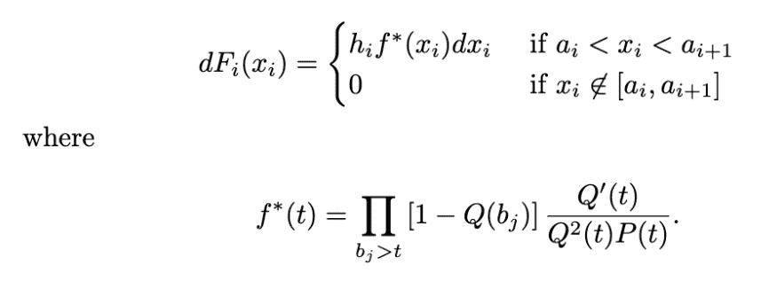
One difficulty is in expressing discontinuous breaks. The definition of $f^*$ is a product over $b_j > t$, but if a $b_j$ lies inside the action interval, that will cause a discontinuity. I don’t know of an easy way to express the $f^*$ product literally as written in sympy (let me know if you know better), so instead I opted to construct a piecewise function manually, which sympy supports nicely.
This results in the following function for building the final $f^*$ for a single action for one player. The piecewise function is to break the action interval into pieces according to the discontinuities introduced by the opponent’s transition times that lie in the same interval.
def f_star(player_action_success: SuccessFn,
           opponent_action_success: SuccessFn,
           variable: Symbol,
           opponent_transition_times: Iterable[float]) -> Expr:
    '''Compute f^* as in Restrepo '57.
    The inputs can be chosen so that the appropriate f^* is built
    for either player. I.e., if we want to compute f^* for player 1,
    player_action_success should correspond to P, opponent_action_success
    to Q, and larger_transition_times to the b_j.
    If the inputs are switched appropriately, f^* is computed for player 2.
    '''
    P: SuccessFn = player_action_success
    Q: SuccessFn = opponent_action_success
    '''
    We compute f^* as a Piecewise function of the following form:
    [prod_{i=1}^m (1-Q(b_i))] * Q'(t) / Q^2(t)P(t)    if t < b_1
    [prod_{i=2}^m (1-Q(b_i))] * Q'(t) / Q^2(t)P(t)    if t < b_2
    [prod_{i=3}^m (1-Q(b_i))] * Q'(t) / Q^2(t)P(t)    if t < b_3
             .
             .
             .
    [1] *  Q'(t) / Q^2(t) P(t)                        if t >= b_m
    '''
    non_product_term = diff(Q(variable), variable) / (Q(variable)**2 * P(variable))
    piecewise_components = []
    for i, b_j in enumerate(opponent_transition_times):
        larger_transition_times = opponent_transition_times[i:]
        product = 1
        for b in larger_transition_times:
            product *= (1 - Q(b))
        term = product * non_product_term
        piecewise_components.append((term, variable < b_j))
    # last term is when there are no larger transition times.
    piecewise_components.append((non_product_term, True))
    return Piecewise(*piecewise_components)
The piecewise components are probability densities, so we can integrate them piecewise to get the cumulative densities. There are a few helpers here to deal with piecewise functions. First, we define a mask_piecewise to modify the sympy-internal representation of a piecewise function to have specified values outside of a fixed interval (the interval on which the action occurs). For a pdf this should be zero, and for a cdf it should be 0 before the action interval and 1 after. There are also some nuanced bits where hidden calls to expr.simplify() allow the integration to happen much faster than otherwise.
def compute_strategy(
        player_action_success: SuccessFn,
        player_transition_times: List[float],
        player_normalizing_constants: List[float],
        opponent_action_success: SuccessFn,
        opponent_transition_times: List[float],
        time_1_point_mass: float = 0) -> Strategy:
    '''
    Given the transition times for a player, compute the action cumulative
    density functions for the optimal strategy of the player.
    '''
    action_distributions = []
    x = Symbol('x', real=True)
    t = Symbol('t', real=True)
    # chop off the last transition time, which is always 1
    opponent_transition_times = [
        x for x in opponent_transition_times if x < 1
    ]
    pairs = subsequent_pairs(player_transition_times)
    for (i, (action_start, action_end)) in enumerate(pairs):
        normalizing_constant = player_normalizing_constants[i]
        dF = normalizing_constant * f_star(
            player_action_success,
            opponent_action_success,
            x,
            opponent_transition_times,
        )
        piece_pdf = mask_piecewise(dF, x, action_start, action_end)
        piece_cdf = integrate(piece_pdf, x, action_start, t)
        piece_cdf = mask_piecewise(
            piece_cdf,
            t,
            action_start,
            action_end,
            before_domain_val=0,
            after_domain_val=1
        )
        action_distributions.append(ActionDistribution(
            support_start=action_start,
            support_end=action_end,
            cumulative_density_function=Lambda((t,), piece_cdf),
        ))
    action_distributions[-1].point_mass = time_1_point_mass
    return Strategy(action_distributions=action_distributions)
def compute_player_strategies(silent_duel_input, intermediate_state, alpha, beta):
    p1_strategy = compute_strategy(
        player_action_success=silent_duel_input.player_1_action_success,
        player_transition_times=intermediate_state.player_1_transition_times,
        player_normalizing_constants=intermediate_state.player_1_normalizing_constants,
        opponent_action_success=silent_duel_input.player_2_action_success,
        opponent_transition_times=intermediate_state.player_2_transition_times,
        time_1_point_mass=alpha,
    )
    p2_strategy = compute_strategy(
        player_action_success=silent_duel_input.player_2_action_success,
        player_transition_times=intermediate_state.player_2_transition_times,
        player_normalizing_constants=intermediate_state.player_2_normalizing_constants,
        opponent_action_success=silent_duel_input.player_1_action_success,
        opponent_transition_times=intermediate_state.player_1_transition_times,
        time_1_point_mass=beta,
    )
    return SilentDuelOutput(p1_strategy=p1_strategy, p2_strategy=p2_strategy)
Note that “Lambda” is a sympy-internal anonymous function declaration that we’re using here to imply functionality. A Lambda also supports function call notation by overloading __call__. This allows the later action distribution to be treated as if it were a function.
Finding the transition times
Next we move on to computing the transition times for a given $\alpha, \beta$. This step is largely the same as in the previous post in this series, but we’re refactoring the code to be simpler and more generic.
The outer loop will construct an intermediate state object, and handle the process that Restrepo describes of “taking the larger parameter” and then computing the next $a_i, b_j$ using the previously saved parameters. There is one caveat, that Restrepo misses when he writes, “for definiteness, we assume that $a_n > b_m$…in the next step…a new $b_m$ is computed…using the single parameter $a_n^*$.” To the best of what I can tell (and experimenting with symmetric examples), when the computed transition times are equal, keeping only one and following Restrepo’s algorithm faithfully will result in an inconsistent output. To the best of what I can tell, this is a minor mistake, and if the transition times are equal then you must keep them both, and not recompute one using the other as a parameter.
def compute_as_and_bs(duel_input: SilentDuelInput,
                      alpha: float = 0,
                      beta: float = 0) -> IntermediateState:
    '''
    Compute the a's and b's for the silent duel, given a fixed
    alpha and beta as input.
    '''
    t = Symbol('t0', nonnegative=True, real=True)
    p1_index = duel_input.player_1_action_count
    p2_index = duel_input.player_2_action_count
    intermediate_state = IntermediateState.new()
    while p1_index > 0 or p2_index > 0:
        # the larger of a_i, b_j is kept as a parameter, then the other will be repeated
        # in the next iteration; e.g., a_{i-1} and b_j (the latter using a_i in its f^*)
        (a_i, b_j, h_i, k_j) = compute_ai_and_bj(
            duel_input, intermediate_state, alpha=alpha, beta=beta
        )
        # there is one exception, if a_i == b_j, then the computation of f^* in the next
        # iteration (I believe) should not include the previously kept parameter. I.e.,
        # in the symmetric version, if a_n is kept and the next computation of b_m uses
        # the previous a_n, then it will produce the wrong value.
        #
        # I resolve this by keeping both parameters when a_i == b_j.
        if abs(a_i - b_j) < EPSILON and p1_index > 0 and p2_index > 0:
            # use the average of the two to avoid roundoff errors
            transition = (a_i + b_j) / 2
            intermediate_state.add_p1(float(transition), float(h_i))
            intermediate_state.add_p2(float(transition), float(k_j))
            p1_index -= 1
            p2_index -= 1
        elif (a_i > b_j and p1_index > 0) or p2_index == 0:
            intermediate_state.add_p1(float(a_i), float(h_i))
            p1_index -= 1
        elif (b_j > a_i and p2_index > 0) or p1_index == 0:
            intermediate_state.add_p2(float(b_j), float(k_j))
            p2_index -= 1
    return intermediate_state
It remains to compute an individual $a_i, b_j$ pair given an intermediate state. We refactored the loop body from the last post into a generic function that works for both $a_n, b_m$ (which need access to $\alpha, \beta$) and lower $a_i, b_j$. With the exception of “simple_f_star” there is nothing new happening here.
def simple_f_star(player_action_success: SuccessFn,
                  opponent_action_success: SuccessFn,
                  variable: Symbol,
                  larger_transition_times: Iterable[float]) -> Expr:
    P: SuccessFn = player_action_success
    Q: SuccessFn = opponent_action_success
    non_product_term = diff(Q(variable), variable) / (Q(variable)**2 * P(variable))
    product = 1
    for b in larger_transition_times:
        product *= (1 - Q(b))
    return product * non_product_term
def compute_ai_and_bj(duel_input: SilentDuelInput,
                      intermediate_state: IntermediateState,
                      alpha: float = 0,
                      beta: float = 0):
    '''
    Compute a pair of a_i and b_j transition times for both players,
    using the intermediate state of the algorithm computed so far.
    This function also computes a_n and b_m when the intermediate_state
    input has no larger transition times for the opposite player. In
    those cases, the integrals and equations being solved are slightly
    different; they include some terms involving alpha and beta. In all
    other cases, the alpha and beta parameters are unused.
    '''
    P: SuccessFn = duel_input.player_1_action_success
    Q: SuccessFn = duel_input.player_2_action_success
    t = Symbol('t0', nonnegative=True, real=True)
    a_i = Symbol('a_i', positive=True, real=True)
    b_j = Symbol('b_j', positive=True, real=True)
    p1_transitions = intermediate_state.player_1_transition_times
    p2_transitions = intermediate_state.player_2_transition_times
    # the left end of the transitions arrays contain the smallest
    # (latest computed) transition time for each player.
    # these are set to 1 for an empty intermediate state, i.e. for a_n, b_m
    a_i_plus_one = p1_transitions[0]
    b_j_plus_one = p2_transitions[0]
    computing_a_n = a_i_plus_one == 1
    computing_b_m = b_j_plus_one == 1
    p1_fstar_parameters = list(p2_transitions)[:-1]  # ignore b_{m+1} = 1
    p1_fstar = simple_f_star(P, Q, t, p1_fstar_parameters)
    # the a_i part
    if computing_a_n:
        p1_integrand = ((1 + alpha) - (1 - alpha) * P(t)) * p1_fstar
        p1_integral_target = 2 * (1 - alpha)
    else:
        p1_integrand = (1 - P(t)) * p1_fstar
        p1_integral_target = 1 / intermediate_state.player_1_normalizing_constants[0]
    a_i_integrated = integrate(p1_integrand, t, a_i, a_i_plus_one)
    a_i = solve_unique_real(
        a_i_integrated - p1_integral_target,
        a_i,
        solution_min=0,
        solution_max=a_i_plus_one
    )
    # the b_j part
    p2_fstar_parameters = list(p1_transitions)[:-1]  # ignore a_{n+1} = 1
    p2_fstar = simple_f_star(Q, P, t, p2_fstar_parameters)
    if computing_b_m:
        p2_integrand = ((1 + beta) - (1 - beta) * Q(t)) * p2_fstar
        p2_integral_target = 2 * (1 - beta)
    else:
        p2_integrand = (1 - Q(t)) * p2_fstar
        p2_integral_target = 1 / intermediate_state.player_2_normalizing_constants[0]
    b_j_integrated = integrate(p2_integrand, t, b_j, b_j_plus_one)
    b_j = solve_unique_real(
        b_j_integrated - p2_integral_target,
        b_j,
        solution_min=0,
        solution_max=b_j_plus_one
    )
    # the h_i part
    h_i_integrated = integrate(p1_fstar, t, a_i, a_i_plus_one)
    h_i_numerator = (1 - alpha) if computing_a_n else 1
    h_i = h_i_numerator / h_i_integrated
    # the k_j part
    k_j_integrated = integrate(p2_fstar, t, b_j, b_j_plus_one)
    k_j_numerator = (1 - beta) if computing_b_m else 1
    k_j = k_j_numerator / k_j_integrated
    return (a_i, b_j, h_i, k_j)
You might be wondering what is going on with “simple_f_star”. Let me save that for the end of the post, as it’s related to how I’m currently stuck in understanding the construction.
Binary searching for alpha and beta
Finally, we need to binary search for the desired output $a_1 = b_1$ as a function of $\alpha, \beta$. Following Restrepo’s claim, we first compute $a_1, b_1$ using $\alpha=0, \beta=0$. If $a_1 > b_1$, then we are looking for a $\beta > 0$, and vice versa for $\alpha$.
To facilitate the binary search, I decided to implement an abstract binary search routine (that only works for floating point domains). You can see the code here. The important part is that it abstracts the test (did you find it?) and the response (no, too low), so that we can have the core of this test be a computation of $a_1, b_1$.
First the non-binary-search bits:
def optimal_strategies(silent_duel_input: SilentDuelInput) -> SilentDuelOutput:
    '''Compute an optimal pair of corresponding strategies for the silent duel problem.'''
    # First compute a's and b's, and check to see if a_1 == b_1, in which case quit.
    intermediate_state = compute_as_and_bs(silent_duel_input, alpha=0, beta=0)
    a1 = intermediate_state.player_1_transition_times[0]
    b1 = intermediate_state.player_2_transition_times[0]
    if abs(a1 - b1) < EPSILON:
        return compute_player_strategies(
            silent_duel_input, intermediate_state, alpha=0, beta=0,
        )
    # Otherwise, binary search for an alpha/beta
    searching_for_beta = b1 < a1
    <snip>
    intermediate_state = compute_as_and_bs(
        silent_duel_input, alpha=final_alpha, beta=final_beta
    )
    player_strategies = compute_player_strategies(
        silent_duel_input, intermediate_state, final_alpha, final_beta
    )
    return player_strategies
The above first checks to see if a search is needed, and in either case uses our previously defined functions to compute the output strategies. The binary search part looks like this:
    if searching_for_beta:
        def test(beta_value):
            new_state = compute_as_and_bs(
                silent_duel_input, alpha=0, beta=beta_value
            )
            new_a1 = new_state.player_1_transition_times[0]
            new_b1 = new_state.player_2_transition_times[0]
            found = abs(new_a1 - new_b1) < EPSILON
            return BinarySearchHint(found=found, tooLow=new_b1 < new_a1)
    else:  # searching for alpha
        def test(alpha_value):
            new_state = compute_as_and_bs(
                silent_duel_input, alpha=alpha_value, beta=0
            )
            new_a1 = new_state.player_1_transition_times[0]
            new_b1 = new_state.player_2_transition_times[0]
            found = abs(new_a1 - new_b1) < EPSILON
            return BinarySearchHint(found=found, tooLow=new_a1 < new_b1)
    search_result = binary_search(
        test, param_min=0, param_max=1, callback=print
    )
    assert search_result.found
    # the optimal (alpha, beta) pair have product zero.
    final_alpha = 0 if searching_for_beta else search_result.value
    final_beta = search_result.value if searching_for_beta else 0
Put it all together
Let’s run the complete construction on some examples. I added a couple of print statements in the code and overloaded __str__ on the dataclasses to help. First we can verify we get the same result as our previous symmetric example:
x = Symbol('x')
P = Lambda((x,), x)
Q = Lambda((x,), x)
duel_input = SilentDuelInput(
    player_1_action_count=3,
    player_2_action_count=3,
    player_1_action_success=P,
    player_2_action_success=Q,
)
print("Input: {}".format(duel_input))
output = optimal_strategies(duel_input)
print(output)
output.validate()
# output is:
Input: SilentDuelInput(player_1_action_count=3, player_2_action_count=3, player_1_action_success=Lambda(_x, _x), player_2_action_success=Lambda(_x, _x))
a_1 = 0.143 b_1 = 0.143
P1:
(0.143, 0.200): dF/dt = Piecewise((0, (t > 0.2) | (t < 0.142857142857143)), (0.083/t**3, t < 0.2))
(0.200, 0.333): dF/dt = Piecewise((0, (t > 0.333333333333333) | (t < 0.2)), (0.13/t**3, t < 0.333333333333333))
(0.333, 1.000): dF/dt = Piecewise((0, (t > 1) | (t < 0.333333333333333)), (0.25/t**3, t < 1))
P2:
(0.143, 0.200): dF/dt = Piecewise((0, (t < 0.2) | (t < 0.142857142857143)), (0.083/t**3, t < 0.2))
(0.200, 0.333): dF/dt = Piecewise((0, (t > 0.333333333333333) | (t < 0.2)), (0.13/t**3, t < 0.333333333333333))
(0.333, 1.000): dF/dt = Piecewise((0, (t > 1) | (t < 0.333333333333333)), (0.25/t**3, t > 1))
Validating P1
Validating. prob_mass=1.00000000000000 point_mass=0
Validating. prob_mass=1.00000000000000 point_mass=0
Validating. prob_mass=1.00000000000000 point_mass=0
Validating P2
Validating. prob_mass=1.00000000000000 point_mass=0
Validating. prob_mass=1.00000000000000 point_mass=0
Validating. prob_mass=1.00000000000000 point_mass=0
This lines up: the players have the same strategy, and the transition times are 1/7, 1/5, and 1/3.
Next up, replace Q = Lambda((x,), x**2), and only have a single action for each player. This should require a binary search, but it will be straightforward to verify manually. I added a callback that prints the bounds during each iteration of the binary search to observe. Also note that sympy integration is quite slow, so this binary search takes a minute or two.
Input: SilentDuelInput(player_1_action_count=1, player_2_action_count=1, player_1_action_success=Lambda(_x, _x), player_2_action_success=Lambda(x, x**2))
a_1 = 0.48109 b_1 = 0.42716
Binary searching for beta
{'current_min': 0, 'current_max': 1, 'tested_value': 0.5}
a_1 = 0.37545 b_1 = 0.65730
{'current_min': 0, 'current_max': 0.5, 'tested_value': 0.25}
a_1 = 0.40168 b_1 = 0.54770
{'current_min': 0, 'current_max': 0.25, 'tested_value': 0.125}
a_1 = 0.41139 b_1 = 0.50000
{'current_min': 0, 'current_max': 0.125, 'tested_value': 0.0625}
a_1 = 0.48109 b_1 = 0.44754
{'current_min': 0.0625, 'current_max': 0.125, 'tested_value': 0.09375}
a_1 = 0.41358 b_1 = 0.48860
{'current_min': 0.0625, 'current_max': 0.09375, 'tested_value': 0.078125}
a_1 = 0.41465 b_1 = 0.48297
{'current_min': 0.0625, 'current_max': 0.078125, 'tested_value': 0.0703125}
a_1 = 0.48109 b_1 = 0.45013
{'current_min': 0.0703125, 'current_max': 0.078125, 'tested_value': 0.07421875}
a_1 = 0.41492 b_1 = 0.48157
{'current_min': 0.0703125, 'current_max': 0.07421875, 'tested_value': 0.072265625}
a_1 = 0.48109 b_1 = 0.45078
{'current_min': 0.072265625, 'current_max': 0.07421875, 'tested_value': 0.0732421875}
a_1 = 0.41498 b_1 = 0.48122
{'current_min': 0.072265625, 'current_max': 0.0732421875, 'tested_value': 0.07275390625}
a_1 = 0.48109 b_1 = 0.45094
{'current_min': 0.07275390625, 'current_max': 0.0732421875, 'tested_value': 0.072998046875}
a_1 = 0.41500 b_1 = 0.48113
{'current_min': 0.07275390625, 'current_max': 0.072998046875, 'tested_value': 0.0728759765625}
a_1 = 0.48109 b_1 = 0.45098
{'current_min': 0.0728759765625, 'current_max': 0.072998046875, 'tested_value': 0.07293701171875}
a_1 = 0.41500 b_1 = 0.48111
{'current_min': 0.0728759765625, 'current_max': 0.07293701171875, 'tested_value': 0.072906494140625}
a_1 = 0.41500 b_1 = 0.48110
{'current_min': 0.0728759765625, 'current_max': 0.072906494140625, 'tested_value': 0.0728912353515625}
a_1 = 0.41501 b_1 = 0.48109
{'current_min': 0.0728759765625, 'current_max': 0.0728912353515625, 'tested_value': 0.07288360595703125}
a_1 = 0.48109 b_1 = 0.45099
{'current_min': 0.07288360595703125, 'current_max': 0.0728912353515625, 'tested_value': 0.07288742065429688}
a_1 = 0.41501 b_1 = 0.48109
{'current_min': 0.07288360595703125, 'current_max': 0.07288742065429688, 'tested_value': 0.07288551330566406}
a_1 = 0.48109 b_1 = 0.45099
{'current_min': 0.07288551330566406, 'current_max': 0.07288742065429688, 'tested_value': 0.07288646697998047}
a_1 = 0.48109 b_1 = 0.45099
{'current_min': 0.07288646697998047, 'current_max': 0.07288742065429688, 'tested_value': 0.07288694381713867}
a_1 = 0.41501 b_1 = 0.48109
{'current_min': 0.07288646697998047, 'current_max': 0.07288694381713867, 'tested_value': 0.07288670539855957}
a_1 = 0.48109 b_1 = 0.45099
{'current_min': 0.07288670539855957, 'current_max': 0.07288694381713867, 'tested_value': 0.07288682460784912}
a_1 = 0.41501 b_1 = 0.48109
{'current_min': 0.07288670539855957, 'current_max': 0.07288682460784912, 'tested_value': 0.07288676500320435}
a_1 = 0.41501 b_1 = 0.48109
{'current_min': 0.07288670539855957, 'current_max': 0.07288676500320435, 'tested_value': 0.07288673520088196}
a_1 = 0.48109 b_1 = 0.45099
{'current_min': 0.07288673520088196, 'current_max': 0.07288676500320435, 'tested_value': 0.07288675010204315}
a_1 = 0.48109 b_1 = 0.45099
{'current_min': 0.07288675010204315, 'current_max': 0.07288676500320435, 'tested_value': 0.07288675755262375}
a_1 = 0.48109 b_1 = 0.45099
{'current_min': 0.07288675755262375, 'current_max': 0.07288676500320435, 'tested_value': 0.07288676127791405}
a_1 = 0.41501 b_1 = 0.48109
{'current_min': 0.07288675755262375, 'current_max': 0.07288676127791405, 'tested_value': 0.0728867594152689}
a_1 = 0.41501 b_1 = 0.48109
{'current_min': 0.07288675755262375, 'current_max': 0.0728867594152689, 'tested_value': 0.07288675848394632}
a_1 = 0.41501 b_1 = 0.48109
{'current_min': 0.07288675755262375, 'current_max': 0.07288675848394632, 'tested_value': 0.07288675801828504}
a_1 = 0.48109 b_1 = 0.45099
{'current_min': 0.07288675801828504, 'current_max': 0.07288675848394632, 'tested_value': 0.07288675825111568}
a_1 = 0.48109 b_1 = 0.45099
{'current_min': 0.07288675825111568, 'current_max': 0.07288675848394632, 'tested_value': 0.072886758367531}
a_1 = 0.41501 b_1 = 0.48109
{'current_min': 0.07288675825111568, 'current_max': 0.072886758367531, 'tested_value': 0.07288675830932334}
a_1 = 0.48109 b_1 = 0.45099
{'current_min': 0.07288675830932334, 'current_max': 0.072886758367531, 'tested_value': 0.07288675833842717}
a_1 = 0.48109 b_1 = 0.45099
{'current_min': 0.07288675833842717, 'current_max': 0.072886758367531, 'tested_value': 0.07288675835297909}
a_1 = 0.48109 b_1 = 0.48109
a_1 = 0.48109 b_1 = 0.48109
P1:
(0.481, 1.000): dF/dt = Piecewise((0, (t > 1) | (t < 0.481089134572278)), (0.38/t**4, t < 1))
P2:
(0.481, 1.000): dF/dt = Piecewise((0, (t > 1) | (t < 0.481089134572086)), (0.35/t**4, t < 1)); Point mass of 0.0728868 at 1.000
Validating P1
Validating. prob_mass=1.00000000000000 point_mass=0
Validating P2
Validating. prob_mass=0.927113241647021 point_mass=0.07288675835297909
This passes the sanity check of the output distributions having probability mass 1. P2 should also have a point mass at the end, because P2’s distribution is $f(x) = x^2$, which has less weight at the beginning and sharply increases at the end. This gives P2 a disadvantage, and pushes their action probability towards the end. According to Restrepo’s theorem, it would be optimal to wait until the end about 7% of the time to guarantee a perfect shot. We can work through the example by hand, and turn the result into a unit test.
Note that we haven’t verified this example is correct by hand. We’re just looking at some sanity checks at this point.
Where it falls apart
At this point I was feeling pretty good, and then the following example shows my implementation is broken:
x = Symbol('x')
P = Lambda((x,), x)
Q = Lambda((x,), x**2)
duel_input = SilentDuelInput(
    player_1_action_count=2,
    player_2_action_count=2,
    player_1_action_success=P,
    player_2_action_success=Q,
)
print("Input: {}".format(duel_input))
output = optimal_strategies(duel_input)
print(output)
output.validate(err_on_fail=False)
The output shows that the resulting probability distribution does not have a total probability mass of 1. I.e., it’s not a distribution. Uh oh.
Input: SilentDuelInput(player_1_action_count=2, player_2_action_count=2, player_1_action_success=Lambda(_x, _x), player_2_action_success=Lambda(x, x**2))
a_1 = 0.34405 b_1 = 0.28087
Binary searching for beta
{'current_min': 0, 'current_max': 1, 'tested_value': 0.5}
a_1 = 0.29894 b_1 = 0.45541
{'current_min': 0, 'current_max': 0.5, 'tested_value': 0.25}
a_1 = 0.32078 b_1 = 0.36181
{'current_min': 0, 'current_max': 0.25, 'tested_value': 0.125}
a_1 = 0.32660 b_1 = 0.34015
{'current_min': 0, 'current_max': 0.125, 'tested_value': 0.0625}
a_1 = 0.34292 b_1 = 0.29023
{'current_min': 0.0625, 'current_max': 0.125, 'tested_value': 0.09375}
a_1 = 0.33530 b_1 = 0.30495
{'current_min': 0.09375, 'current_max': 0.125, 'tested_value': 0.109375}
a_1 = 0.32726 b_1 = 0.33741
{'current_min': 0.09375, 'current_max': 0.109375, 'tested_value': 0.1015625}
a_1 = 0.32758 b_1 = 0.33604
{'current_min': 0.09375, 'current_max': 0.1015625, 'tested_value': 0.09765625}
a_1 = 0.32774 b_1 = 0.33535
{'current_min': 0.09375, 'current_max': 0.09765625, 'tested_value': 0.095703125}
a_1 = 0.33524 b_1 = 0.30526
{'current_min': 0.095703125, 'current_max': 0.09765625, 'tested_value': 0.0966796875}
a_1 = 0.33520 b_1 = 0.30542
{'current_min': 0.0966796875, 'current_max': 0.09765625, 'tested_value': 0.09716796875}
a_1 = 0.32776 b_1 = 0.33526
{'current_min': 0.0966796875, 'current_max': 0.09716796875, 'tested_value': 0.096923828125}
a_1 = 0.32777 b_1 = 0.33522
{'current_min': 0.0966796875, 'current_max': 0.096923828125, 'tested_value': 0.0968017578125}
a_1 = 0.33520 b_1 = 0.30544
{'current_min': 0.0968017578125, 'current_max': 0.096923828125, 'tested_value': 0.09686279296875}
a_1 = 0.32777 b_1 = 0.33521
{'current_min': 0.0968017578125, 'current_max': 0.09686279296875, 'tested_value': 0.096832275390625}
a_1 = 0.32777 b_1 = 0.33521
{'current_min': 0.0968017578125, 'current_max': 0.096832275390625, 'tested_value': 0.0968170166015625}
a_1 = 0.32777 b_1 = 0.33520
{'current_min': 0.0968017578125, 'current_max': 0.0968170166015625, 'tested_value': 0.09680938720703125}
a_1 = 0.32777 b_1 = 0.33520
{'current_min': 0.0968017578125, 'current_max': 0.09680938720703125, 'tested_value': 0.09680557250976562}
a_1 = 0.32777 b_1 = 0.33520
{'current_min': 0.0968017578125, 'current_max': 0.09680557250976562, 'tested_value': 0.09680366516113281}
a_1 = 0.33520 b_1 = 0.30544
{'current_min': 0.09680366516113281, 'current_max': 0.09680557250976562, 'tested_value': 0.09680461883544922}
a_1 = 0.32777 b_1 = 0.33520
{'current_min': 0.09680366516113281, 'current_max': 0.09680461883544922, 'tested_value': 0.09680414199829102}
a_1 = 0.32777 b_1 = 0.33520
{'current_min': 0.09680366516113281, 'current_max': 0.09680414199829102, 'tested_value': 0.09680390357971191}
a_1 = 0.32777 b_1 = 0.33520
{'current_min': 0.09680366516113281, 'current_max': 0.09680390357971191, 'tested_value': 0.09680378437042236}
a_1 = 0.33520 b_1 = 0.30544
{'current_min': 0.09680378437042236, 'current_max': 0.09680390357971191, 'tested_value': 0.09680384397506714}
a_1 = 0.33520 b_1 = 0.30544
{'current_min': 0.09680384397506714, 'current_max': 0.09680390357971191, 'tested_value': 0.09680387377738953}
a_1 = 0.32777 b_1 = 0.33520
{'current_min': 0.09680384397506714, 'current_max': 0.09680387377738953, 'tested_value': 0.09680385887622833}
a_1 = 0.32777 b_1 = 0.33520
{'current_min': 0.09680384397506714, 'current_max': 0.09680385887622833, 'tested_value': 0.09680385142564774}
a_1 = 0.32777 b_1 = 0.33520
{'current_min': 0.09680384397506714, 'current_max': 0.09680385142564774, 'tested_value': 0.09680384770035744}
a_1 = 0.33520 b_1 = 0.30544
{'current_min': 0.09680384770035744, 'current_max': 0.09680385142564774, 'tested_value': 0.09680384956300259}
a_1 = 0.32777 b_1 = 0.33520
{'current_min': 0.09680384770035744, 'current_max': 0.09680384956300259, 'tested_value': 0.09680384863168001}
a_1 = 0.32777 b_1 = 0.33520
{'current_min': 0.09680384770035744, 'current_max': 0.09680384863168001, 'tested_value': 0.09680384816601872}
a_1 = 0.32777 b_1 = 0.33520
{'current_min': 0.09680384770035744, 'current_max': 0.09680384816601872, 'tested_value': 0.09680384793318808}
a_1 = 0.32777 b_1 = 0.33520
{'current_min': 0.09680384770035744, 'current_max': 0.09680384793318808, 'tested_value': 0.09680384781677276}
a_1 = 0.32777 b_1 = 0.33520
{'current_min': 0.09680384770035744, 'current_max': 0.09680384781677276, 'tested_value': 0.0968038477585651}
a_1 = 0.33520 b_1 = 0.30544
{'current_min': 0.0968038477585651, 'current_max': 0.09680384781677276, 'tested_value': 0.09680384778766893}
a_1 = 0.33520 b_1 = 0.33520
a_1 = 0.33520 b_1 = 0.33520
deque([0.33520049631043414, 0.45303439059299566, 1])
deque([0.33520049631043414, 0.4897058985296734, 1])
P1:
(0.335, 0.453): dF/dt = Piecewise((0, t < 0.335200496310434), (0.19/t**4, t < 0.453034390592996), (0, t > 0.453034390592996))
(0.453, 1.000): dF/dt = Piecewise((0, t < 0.453034390592996), (0.31/t**4, t < 0.489705898529673), (0.4/t**4, t < 1), (0, t > 1))
P2:
(0.335, 0.490): dF/dt = Piecewise((0, t < 0.335200496310434), (0.17/t**4, t < 0.453034390592996), (0.3/t**4, t < 0.489705898529673), (0, t > 0.489705898529673))
(0.490, 1.000): dF/dt = Piecewise((0, t < 0.489705898529673), (0.36/t**4, t < 1), (0, t > 1)); Point mass of 0.0968038 at 1.000
Validating P1
Validating. prob_mass=0.999999999999130 point_mass=0
Validating. prob_mass=1.24303353980824 point_mass=0   INVALID
Probability distribution does not have mass 1: (0.453, 1.000): dF/dt = Piecewise((0, t < 0.453034390592996), (0.31/t**4, t < 0.489705898529673), (0.4/t**4, t < 1), (0, t > 1))
Validating P2
Validating. prob_mass=1.10285404591706 point_mass=0   INVALID
Probability distribution does not have mass 1: (0.335, 0.490): dF/dt = Piecewise((0, t < 0.335200496310434), (0.17/t**4, t < 0.453034390592996), (0.3/t**4, t < 0.489705898529673), (0, t > 0.489705898529673))
Validating. prob_mass=0.903196152212331 point_mass=0.09680384778766893
What’s fundamentally different about this example? The central thing I can tell is that this is the simplest example for which player 1 has an action that has a player 2 transition time in the middle. It’s this action:
(0.453, 1.000): dF/dt = Piecewise((0, t < 0.453034390592996), (0.31/t**4, t < 0.489705898529673), (0.4/t**4, t < 1), (0, t > 1))
...
Validating. prob_mass=1.24303353980824 point_mass=0   INVALID
This is where the discontinuity of $f^*$ actually matters. In the previous example either there was only one action, and by design the starting times of the action ranges are equal, or else the game was symmetric, so that the players had the same action range endpoints.
In my first implementation, I had actually ignored the discontinuities entirely, and because the game was symmetric it didn’t impact the output distributions. This is what’s currently in the code as “simple_f_star.” Neither player’s action transitions fell inside the bounds of any of the other player’s action ranges, and so I missed that the discontinuity was important.
In any event, in the three years since I first worked on this, I haven’t been able to figure out what I did wrong. I probably won’t come back to this problem for a while, and in the mean time perhaps some nice reader has the patience to figure it out. You can see a log of my confusion in this GitHub issue, and some of the strange workarounds I tried to get it to work.
Want to respond? Send me an email, post a webmention, or find me elsewhere on the internet.